
Introduction to survival analysis
Understanding the dynamics of survival times in clinical settings is important to both medical practitioners and patients. In statistics, time-to-event analysis models a continuous random variable \(T\), which represents the duration of a state. If the state is “being alive”, then the time to event is mortality, and we refer to it as survival anaylsis. If \(t\) is a given realization of \(T\), then we are conceptually interested in modelling \(P_\theta(T>t|X)\), indexed by some parametric distribution \(\theta\) and conditional on some baseline covariates \(X\). If a patient has the state of being alive with cancer, then survival analysis answers the question: what is the probability that life expectancy will exceed \(t\) months given your features \(X\) (age, gender, genotype, etc) and underlying biological condition[1].
If \(T\) is a continuous random variable, then it has a CDF and PDF of course, but in survival analysis we are also interested in two other functions (dropping the subscripts/conditional variables for notational simplicity):
- Survival function: \(S(t)=1-F(t)\). Probability of being alive at time \(t\).
- Hazard function: \(h(t)=\frac{f(t)}{S(t)}\). The rate of change of risk, given you are alive at \(t\).
Visualizing each term in R provides a useful way to understand what each function represents. Assume that \(T \sim \text{Exp}(\theta)\) distribution.
# Use theta=2
F.t <- function(t) { pexp(t,rate=2) }
f.t <- function(t) { dexp(t,rate=2) }
S.t <- function(t) { 1 - F.t(t) }
h.t <- function(t) { f.t(t)/S.t(t) }
# Generate data
dat1 <- data.frame(t=seq(0,2,0.1)) %>%
          mutate(Ft=F.t(t),ft=f.t(t),St=S.t(t),ht=h.t(t)) %>%
          gather(dist,val,-t) %>% tbl_df %>% mutate(dist=gsub('t','[t]',dist))
# Plot
ggplot(dat1,aes(x=t,y=val,color=dist)) + geom_line(size=1,show.legend=F) +
  facet_wrap(~dist,scales='free_y',labeller=label_parsed) + theme_cowplot(font_size = 6) +
  labs(x='Time') + ggtitle('Survival analysis functions') + theme(axis.title.y=element_blank())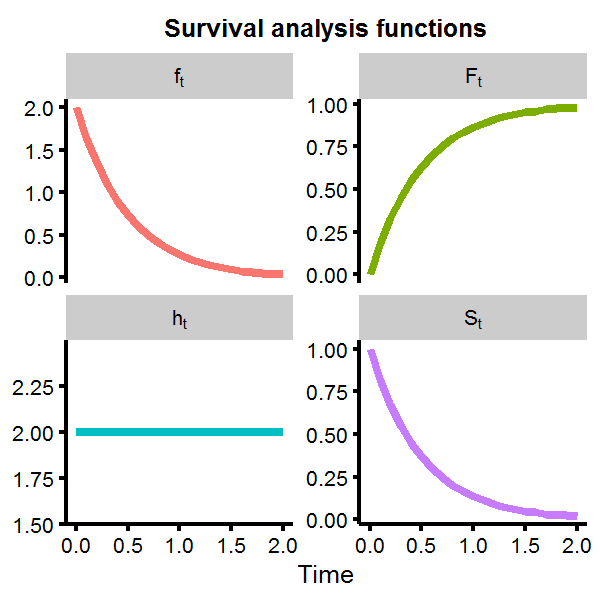
We can see that the survival function rapidly approaches zero as time increases, with the probability of living longer than \(t>2\) almost nill. However, the hazard function is flat at \(h(t)=2\). This is not unexpected, as the exponential distribution is known to give a constant hazard function, meaning that given that you have made it to some point \(t_1\) or \(t_2\), the probability of mortality in the next moment is the same for both cases, which is another way of saying the exponential distribution is memoryless.
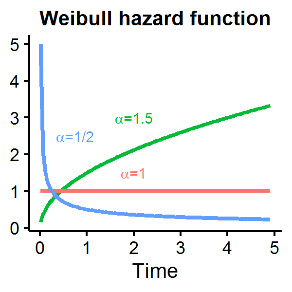
As a constant hazard rate is a strong modelling assumption, alternative distributions for the duration measure are often used in the literature including the Weibull distribution which permits an increasing, decreasing, or constant hazard rate depending on \(\alpha\):
\(T \sim\) Weibull distribution
- \(F(t|\theta,\alpha)=1-\exp[-(\theta t)^\alpha]\)
- \(S(t|\theta,\alpha)=\exp[-(\theta t)^\alpha]\)
- \(h(t|\theta,\alpha)=\alpha\theta^\alpha t^{\alpha-1}\)
Let’s see how the Weibull hazard function looks for different parameterizations of \(\alpha\) with \(\theta=1\). When \(\alpha=1\) the hazard function is constant over time, but is decreasing (increasing) if \(\alpha\) is less (greater) than one.
A distribution with covariates
If \(\theta\) parameterizes our distribution, then to introduce covariates which influence survival times we can simply rewrite \(X\beta=\theta\) such that each individual \(i\) and \(j\) will have a different hazard rate if their baseline covariates differ[2]. We can model the log likelihood as:
\[\begin{aligned} l(\boldsymbol t | \beta,\alpha) &=\sum_{i=1}^n \log f(t_i | X_i,\beta,\alpha ) \\ &= \sum_{i=1}^n \log h(t_i | X_i,\beta,\alpha ) + \sum_{i=1}^n \log S(t_i | X_i,\beta,\alpha ) \end{aligned}\]We will generate a simple example with 20 individuals, using a Weibull distribution with \(\alpha=1.5\), and an intercept and dummy covariates. The dummy variable can be thought of as a receiving a treatment or not. Also note that the weibull functions in R use a scale parameter which is \(1/\theta\).
set.seed(1)
n <- 20 # Number of patients
alpha <- 1.5
X <- data.frame(patient=str_c('id',1:n),iota=rep(1,n),treatment=sample(c(0,1),n,replace=T))
beta <- c(1,-2/3)
# Generate observed survival times
t.obs <- rweibull(n,shape=alpha,scale=1/(as.matrix(X[,c('iota','treatment')])%*%beta))
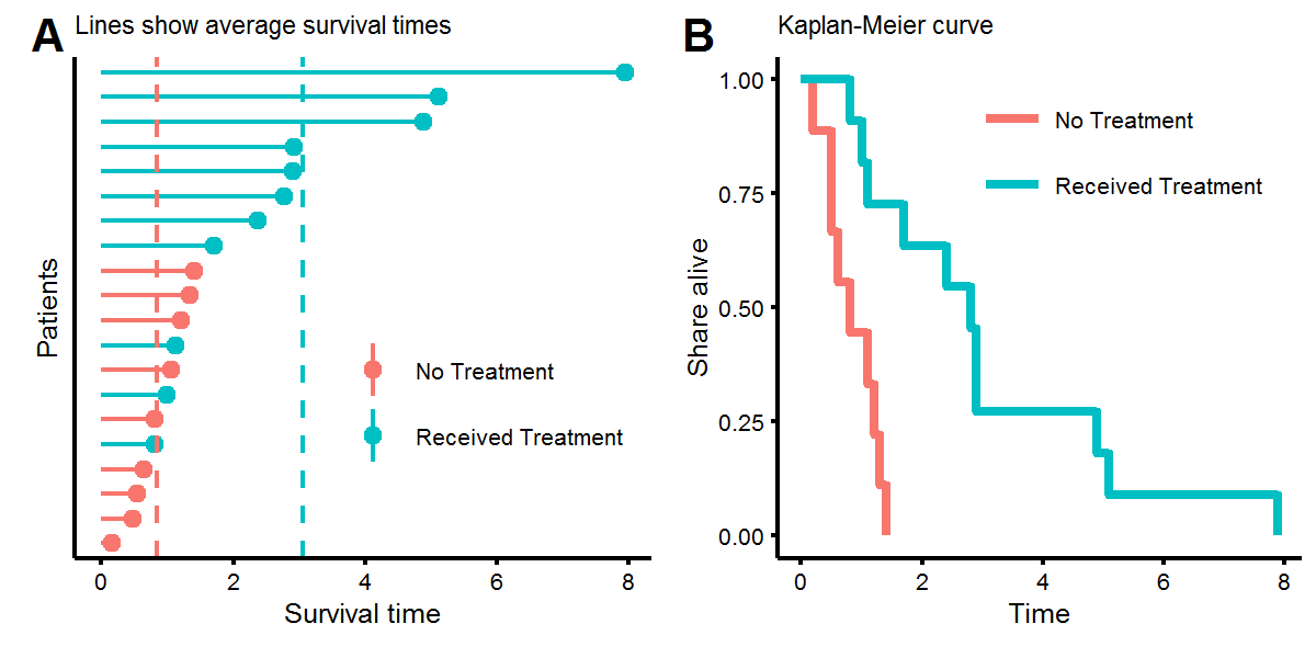
X.obs <- cbind(t.obs,X)Let’s look at the distribution of our survival times. In figure A below we see that while some people who didn’t receive the treatment lived longer than those who did, on average, receiving the treatment increased survival times from around \(t=1\) to \(t=3\). This was result was engineered by setting the coefficients to \(\beta=[1,-2/3]^T\). Figure B, known as a Kaplan-Meier (KM) plot, shows a non-parametric estimate of survival times. Every time there is a step downwards, this represents the death of a patient. KM plots are popular due to their the visual interpretability, as one can ask (1) what share of the treatment group is alive after four units of time, or (2) at what time have half of the patients died?
To find the maximum likelihood estimate of the data we can use the optim function in base R (this is easier than writing a Newton-Raphson algorithm). We see that our parameter estimates are fairly close, especially with only twenty observations to perform the inference.
# Log-likelihood
llik <- function(theta,t,dat) {
  t1 <- theta[1] # alpha
  t2 <- theta[2] # beta_0
  t3 <- theta[3] # beta_1
  fv <- dat %*% rbind(t2,t3)
  -1* ( sum( log(t1) + t1*log(fv) + (t1-1)*log(t) ) + sum( -(fv*t)^t1  ) )
}
# Optimize
mlik <- optim(par=c(1,1,0),fn=llik,dat=cbind(1,X.obs$treatment),t=X.obs$t.obs)$par
data.frame(Parameters=c('alpha','beta[0]','beta[1]'),
           True.Value=round(c(alpha,beta),1),Maximum.Likelihood=round(mlik,1))
## Parameters True.Value Maximum.Likelihood
## 1 alpha 1.5 1.8
## 2 beta[0] 1.0 1.1
## 3 beta[1] -0.7 -0.8Notice that one can write the hazard function for the Weibull distribution as \(h(t_i|X_i,\beta,\alpha)=g_1(X_i)g_2(t)\), with \(g_2\) known as the baseline hazard function, so that ratio of two hazard functions between person \(i\) and \(j\) is going to indepdent of the survival time:
\(\frac{h(t_i,X_i)}{h(t_j,X_j)}=\Big(\frac{X_i\beta}{X_j\beta}\Big)^\alpha\)
This result, known as the proportional hazards assumption, allows for the estimates of the parameters contained within \(g_1\) to be estimated independently of \(g_2\), using a method called partial likelihood, which will not be discussed here, but is the approach used by the Cox proportional hazazrd model - the default model used in survival analysis.
Cencoring
Until this point we have only seen observations where the event has occured, meaning we know when a patient’s state began (what is labelled as time zero) and when mortality occured. However, in clinical settings we will not get to observe the event of interest for every patient for several reasons including loss to follow up and insufficient measurement time. Using the previously generated data, we will randomly censor half of the observations by selecting with uniform probability from their true survival time. Note that there are several types of censoring that can occur, but we will use observations which are:
- Right censored: The observed time is as least as large as the eventual survival time.
- Independently censored: Survival time is independent of the censoring event.
Throughout this post, the word censoring will be used for notational simplicity instead of writing “Type II (independent) right-censoring”.
set.seed(1)
# Select with uniform probality the time to event
censor.obs <- X.obs %>% sample_n(10) %>% rowwise() %>%
mutate(t.true=t.obs,t.obs=runif(1,min=0,max=t.obs),censor=T)
censor.obs <- rbind(censor.obs,X.obs %>%
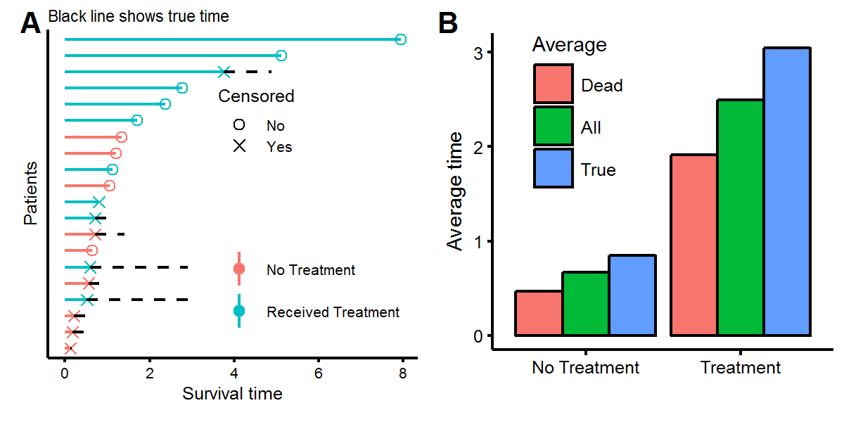
filter(!(patient %in% censor.obs$patient)) %>% mutate(censor=F,t.true=t.obs))We can now visualize the data, showing what we “observe” as the statistician, but also what the true time would have been had we been able to continue observing the patients for longer. Figure A below shows the same twenty patients as before, but with half having censored observations, meaning that these patients are alive (or had an unknown status) at the time of measurement. Using the survival times of either the deceased patients or all the patients will give an underestimate of the true survival times (figure B) because the patients with censored observations will live, on average, for more time.
To perform inference with censored data, the likelihood function will need to account for both censored (\(C\)) and uncensored (\(U\)) observations. If a value is censored, then the density of its observation is not \(f(t)\) but rather \(P(T>t)=S(t)\).
\[\begin{aligned} l(\boldsymbol t | \beta,\alpha) &= \sum_{i\in C} \log f(t_i | X_i,\beta,\alpha ) + \sum_{j \in U} \log S(t_j | X_j,\beta,\alpha ) \end{aligned}\]Next, we’ll generate a larger data set (\(n=100\)) with 50% of the obsersations independently censored, and then use the log-likelihood formulation above to estimate the \(\alpha\) and \(\beta\) parameters.
n <- 100
set.seed(1)
X <- data.frame(iota=1,treatment=rbernoulli(n)*1) %>% as.matrix
# Generate censored observations with probability 50%
rw <- rweibull(n,shape=alpha,scale=1 / (X %*% beta))
rc <- runif(n,min=0,max=rw)
is.censored <- rbernoulli(n)
dat <- tbl_df(data.frame(t.obs=ifelse(is.censored,rc,rw),t.true=rw,censored=is.censored,X))

# Log-likelihood with censoring
# theta <- c(1,1,-0.5);t=dat$t.obs;censor=dat$censored;dat=cbind(1,dat$treatment)
llik.censor <- function(theta,t,censor,dat) {
  t1 <- theta[1] # alpha
  t2 <- theta[2] # beta_0
  t3 <- theta[3] # beta_1
  # Find which observations are censored
  C.obs <- which(censor)
  U.obs <- which(!censor)
  # Calculate observations beforehand
  fv <- dat %*% rbind(t2,t3)
  fv.C <- fv[C.obs]; fv.U <- fv[U.obs]
  t.C <- t[C.obs]; t.U <- t[U.obs]
  # Calculate
  -1*( sum( log(t1) + t1*log(fv.U) + (t1-1)*log(t.U) ) + sum( -(fv.U*t.U)^t1  ) + sum( -(fv.C*t.C)^t1  )  )
}
# Optimize
mlik.censor <- optim(par=c(1,0.5,0),fn=llik.censor,t=dat$t.obs,censor=dat$censored,dat=cbind(1,dat$treatment))$par
mlik.wrong <- optim(par=c(1,0.5,0),fn=llik,t=dat$t.obs,dat=cbind(1,dat$treatment))$par

data.frame(Parameters=c('alpha','beta[0]','beta[1]'),
           True.Value=round(c(alpha,beta),1),
           'ML with censoring'=round(mlik.censor,1),
           'ML without censoring'=round(mlik.wrong,1))
## Parameters True.Value ML.with.censoring ML.without.censoring
## 1 alpha 1.5 1.7 1.2
## 2 beta[0] 1.0 0.9 1.5
## 3 beta[1] -0.7 -0.6 -1.0With the parameter estimates, we can now estimate what the average survival time for patients with and without the treatment would be, noting that the mean for a Weibull distribution is \(\frac{1}{\theta}\Gamma(1+1/\alpha)\).
a <- mlik.censor[1]
b1 <- mlik.censor[2]
b2 <- mlik.censor[3]
theta.treat <- sum(c(1,1)*c(b1,b2))
theta.notreat <- sum(c(1,0)*c(b1,b2))
mu.treat <- (1/theta.treat)*gamma(1+1/a)
mu.notreat <- (1/theta.notreat)*gamma(1+1/a)
xbar <- dat %>% group_by(treatment) %>% summarise(xbar=mean(t.obs))
x.all <- dat %>% group_by(treatment) %>% summarise(xbar=mean(t.true))
# Print
data.frame(Treatment=c('Yes','No'),Inference=c(mu.treat,mu.notreat),
           'Sample-mean'=c(rev(xbar$xbar)),'True sample-mean'=c(rev(x.all$xbar))) %>%
  mutate_if(is.numeric,funs(round(.,1)))
## Treatment Inference Sample.mean True.sample.mean
## 1 Yes 3 2.2 2.5
## 2 No 1 0.6 0.9While our inference shows that individuals should live longer than what we observe, it seems “too high” compared to the sample mean we would have observed had the observations not been censored. This is due to the problems of finite sample bias, in maximum likelihood estimators. Correcting for this is beyond the scope of this analysis. Overall, this post has highlighted the importance of survival models in statistics: (1) they provide a way to estimate the distribution of survival times for different patients using variation in baseline covariates, and (2) they are able to extract information from both censored and uncensored observations to perform inference.
-
If there were two data sets of survival times with patient cohorts of breast and pancreatic cancer, then we would expect that probability of survival would be lower in the latter group, even if patients with breast/pancreatic cancer had the same covariate values, simply because pancreatic cancer is known to be a more aggressive cancer. ↩
-
Note that this is only saying that \(f_i\neq f_j\) because \(X_i\neq X_j\) which is different than \(\beta_i \neq \beta_j\). The former assumes baseline covariates cause differences in expected survival outcomes, whereas the latter is saying that for the same set of covariate values, survival times will differ between individuals. While simple survival models, and the type used in this post, assume that \(\beta\) is the same between individuals, this is becoming a more reasonable assumption as the quality of biomedical data sets increases, especially with access to genomic data. For example, if one of the covariates in a breast cancer study is whether a patient received a selective estrogen receptor modulator, than we would expect \(\beta\) to differ in its effects depending on the underlying genetic profile of tumor. Whereas if we had access to gene expression for genes such as \(her2\) or \(brca1\) this should control for the different efficacies of treatment across gene types. ↩