
Machine learning and causal inference
Introduction
Machine learning and traditional statistical inference have, until very recently, been running along separate tracks. In broad strokes, machine learning researchers were interested in developing algorithms which maximized predictive accuracy. Natural processes were seen as a black box which could be approximated by creative data mining procedures. This approach has been termed the “algorithmic modelling culture” (Breiman 2001).
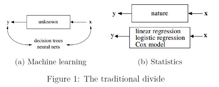
In contrast, the statistical approach posits that nature’s black box is actually a stochastic model that determines what we observe: \(\text{outcomes}=f(\text{data},\text{parameters},\text{noise})\). The objective of the statistician is to perform inference and learn something about the values of these parameters and their associated uncertainty. The goal is to be able to make statements about how the natural world works. Using Breiman’s terms again, we can refer to this as the “data/statistical modelling culture”.
Machine learning has proved incredibly successful in many fields such as recommender systems, language translation, or image recognition. Predictive algorithms in these domains have changed rapidly over time as computing power has expanded and new techniques were discovered. When Google Translate changes their deep learning architecture to improve translation accuracy their results are judged on the quality of the output, rather than whether the internal syntax representations learned by the neural network reflect the true nature of semantics.
In fields such as epidemiology, economics, and most of the social sciences, an explicit modelling form is taken, (usually) indexed by a parametric distribution which we are interested in performing inference on. Whether or not these parameters are themselves stochastic[1], the model results are meant to be interpretative. Whereas algorithmic modelers would be happy to have a data set labelled \(X_1,\dots,X_n\), the data modelers want to be able to link the model results to actual covariates of interest: \(\text{treatment}_1,\dots,\text{age}\). In other words, we need to know both whether the patient will get better and whether \(\text{treatment}_1\) was in any was responsible for this[2].
As the size and richness of data sets have grown in fields traditionally under the purview of statistical modelers, and as machine learning researchers have been asked to apply their techniques to a broader array of problems, these fields are beginning to merge. For example, data mining techniques developed for data sets where the number of features vastly exceeds observations are now de rigueur in many areas, such as genomics. At the same time, machine learning techniques based on model selection for out-of-sample accuracy have proved insufficient at determining what will happen when a fundamental change in the underlying structure occurs. In the machine learning parlance, these models are unable to “translate” their functional approximations to a new domain (Dai and Yu 2008). Examples of which include a change in auction design for selling ad space or some policy treatment.
A new synthesis between the machine learning and statistical modelling approaches is currently being developed with an emphasis on causal inference in high-dimensional setting (see (Athey and Imbens 2016) or (Belloni and Hansen 2015)). Machine learning provides the techniques required for handling large and over-determined data sets, and statistics provides the means for performing inference and defining a causal framework for a choice set of features (see (Rosembaum and Rubin 1983) and (Holland 1986)). This summary document discusses some of the major themes in machine learning and statistics with the goal of describing a framework for performing causal inference in high dimensional space. Such a framework could be applied to a large clinical data set, with possibly more variables than observations, in which a researcher is interested in measuring how a treatment variable impacts some clinical outcome. The rest of this monograph is structured as follows: four relevant background topics from machine learning are covered, followed by two promising and recently-developed modelling strategies for causal inference in high dimensional settings.
Background #1: When features exceed observations (\(p \gg N\))
While data sets have been getting longer, they have also been getting fatter. When the number of variables (or features) exceeds the number of observations, we refer to this as the \(p \gg N\) problem. The first, and terminal, problem this poses to traditional statistical models is that they will quickly “blow up”. Equation (1) shows the matrix operations which determine the parameter weights \(\boldsymbol\beta\) of a traditional linear model.
\[\begin{align*} \hat{\boldsymbol\beta} &= (\textbf{X}^T\textbf{X})^{-1} \textbf{X}^T \textbf{y} \hspace{1cm} (1) \end{align*}\]To be able to efficiently estimate \((\textbf{X}^T\textbf{X})^{-1}\), which is a sort of uncentered scatter matrix, the number of columns cannot exceed the number rows. As \(p \to n\), the linear model begins to perfectly represent the data by reparameterizing the observations into some linear combination of the coefficients. In other words, it is a “saturated model”. To deal with this problem, almost all machine learning models use some form of regularization, which is a way of penalizing model complexity to ensure that the model parameters do not perfectly fit the “noise” of the data. If the outcome of interest \(\textbf{y}\) is a continuous variable, instead of minimizing the residual sum of squares (RSS), a regularized model will trade off minimizing the RSS with some measure of model complexity. This is sometimes called the penalized residual sum of squares (PRSS), as shown in equation (2) where \(J\) is some functional that measures model complexity and \(\lambda\) is the weight placed against such complexity.
\[\begin{align*} PRSS(\boldsymbol\beta) = \arg\min_{\boldsymbol\beta} \hspace{2mm} \| \textbf{y} - f(\boldsymbol\beta) \|^2 + \lambda J(f(\boldsymbol\beta)) \hspace{1cm} (2) \end{align*}\]The tradeoff between in-sample accuracy and model complexity is also known as the bias-variance tradeoff. When the objective function is to minimize the expected RSS, this is tradeoff can be explicitly modeled in a closed form:
\[\text{MSE}(f(\boldsymbol\beta)) = \text{Bias}(f(\boldsymbol\beta))^2 + \text{Var}(f(\boldsymbol\beta))\]To highlight one model, ridge regression, a time-honored approach to regularization (Hoerl 1962), uses the L2-norm of the coefficient weights as the measure of model complexity. The minimization problem can therefore be stated as:
\[\begin{align*} \boldsymbol\beta_{\text{Ridge}} &= \arg\min_{\boldsymbol\beta} \hspace{2mm} \| \textbf{y} - \textbf{X}\boldsymbol\beta\|^2 + \lambda \|\boldsymbol\beta\|^2_2 \\ &= \arg\min_{\boldsymbol\beta} \hspace{2mm} RSS(\boldsymbol\beta) + \lambda \sum_{i=1}^p \beta_i^2 \end{align*}\]The solution to the ridge regression problem effectively involves shrinking each coefficient towards zero. In this sense, ridge regression does not appeal to sparsity and keeps all of the parameters. In other situations, we may want the model selection procedure to throw away covariates rather than just shrink them. A Monte Carlo experiment can further elucidate the necessity of some form of regularization in a high dimensional setting. A range of penalized models will be estimated in an environment where features exceed observations by 5:2.
- Generate a model where \(\textbf{y}=\textbf{X}\boldsymbol\beta + \boldsymbol\epsilon\), where \(n=1100\), \(p=250\), and \(\boldsymbol\epsilon\) is Gaussian white noise.
- Generate the values of \(\boldsymbol\beta\) such that \(\beta_k \sim N(0,[1/k]^r)\), where \(r={0.5,1}\). In other words, each coefficient has a causal impact on the outcomes, but the impact of the \(k^{th}\) model parameter approaches zero either linearly \(r=0.5\) or geometrically \(r=1\) (hence a small share of covariates cause most of the variation in the outcome).
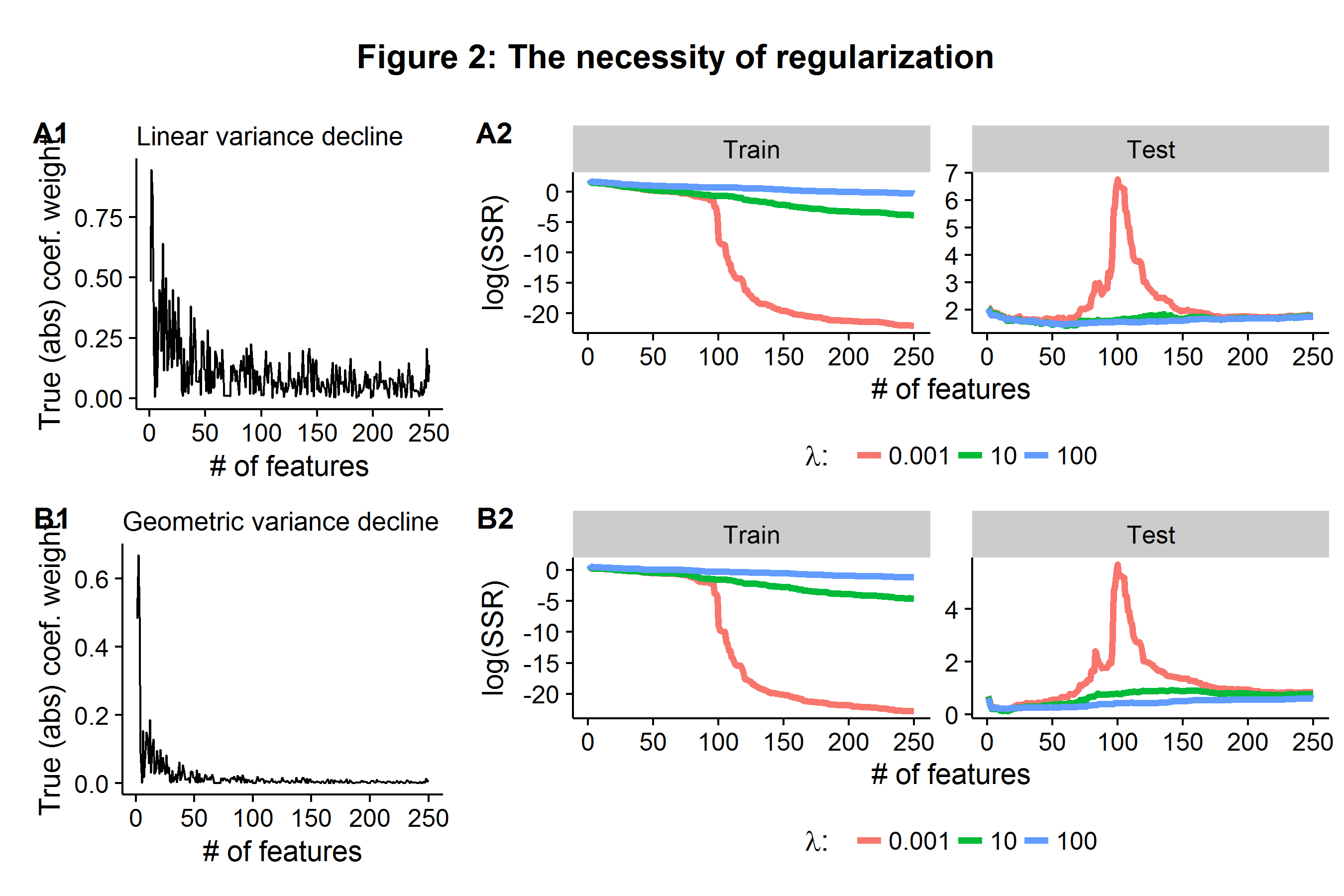
- Estimate three ridge regression models using only the first \(n_1=100\) observations (the training stage) for three values of \(\lambda={0.001,10,100 }\), where \(\lambda=0.001\) is effectively the classical linear model because almost no weight is placed against model complexity.
- Compare each model’s accuracy on the held-out \(n_2=1000\) observations (the testing stage) as each model is given more and more variables (and hence parameters) in the initial training stage where \(n_1=100\).
Each row in Figure 2 below represents presents the same data generating process, but varies in whether the (true) coefficient weight impacts are declining linearly or geometrically (A1 and B1). In the training sample, once the \(\lambda=0.001\) model is fed \(p=100\) features it is able to (almost) perfectly represent the data and the RSS falls close to zero. However, when these estimated parameters are applied to the held-out data, the error explodes because the coefficient weights were tuned to the noise of the training data set. In contrast, the models which penalized model complexity are able to stabilize the average error rate as the model is deployed to the held-out test data set, even when they are given more features than observations in the training stage. In the case of geometrically declining (true) coefficient weights, the \(\lambda=100\) model is able to maintain the lowest test error even as the number of features far exceeds the number of observations it was trained on.
Background #2: Model selection for accuracy
While model selection/regularization becomes inevitable as \(p \to n\), the question of determining how much regularization is appropriate becomes paramount. In the previous example we saw that \(\lambda=100\) outperformed the other two regularization parameters, but was this the best choice of \(\lambda\)? Furthermore, the previous example was able to use a “hidden” set of data to measure accuracy because we knew what the underlying data generating process was. As most machine learning models contain hyperparameters (such as \(\lambda\) for ridge regression), when dealing with real-world data sets, researchers often use k-fold cross validation (CV) to perform model selection. For a given hyperparameter the CV algorithm is as follows:
- Partition the data into \(k\) (roughly) equal blocks.
- Fit a given model (e.g. ridge regression) on \(k-1\) of the other blocks.
- Use the model parameters from Step 2 to make predictions for the remaining \(k^{th}\) block.
- Record model accuracy and repeat Steps 2 and 3 for all \(k\) blocks.
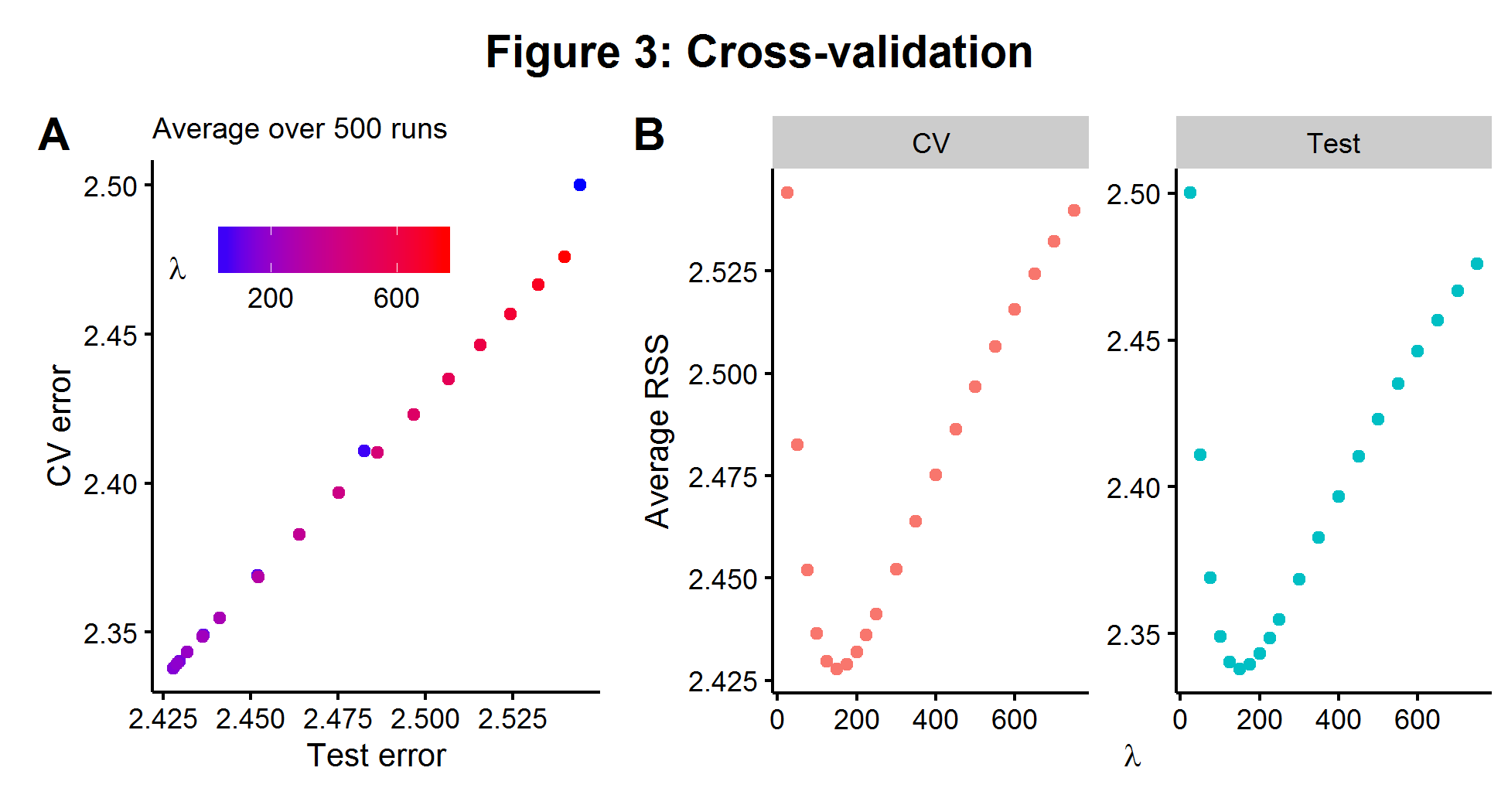
The average CV model error can be compared over a range of hyperparameter choices and the one which minimizes the CV error is chosen. CV is highly appealing because it is both conceptually simple and can be used on any model which makes predictions. Using the same model described in the section above, we fit a range of \(\lambda\)’s with 5-fold cross validation. In Figure 3A below, we see that over 500 simulations there is an almost perfect relationship between the CV error rate on the \(n_1=100\) data and the error rate we would be able to measure if we had access to the \(n_2=1000\) held out data (on average). The two plots in Figure 3B show that the value of \(\lambda\) which minimizes the CV error is the same for the larger test data set. The results below show the power of cross-validation to be able to “approximate” the true bias-variance tradeoff of a hidden data set by chopping up a smaller data set that we can see and iterating over it.
Background #3: The curse of dimensionality
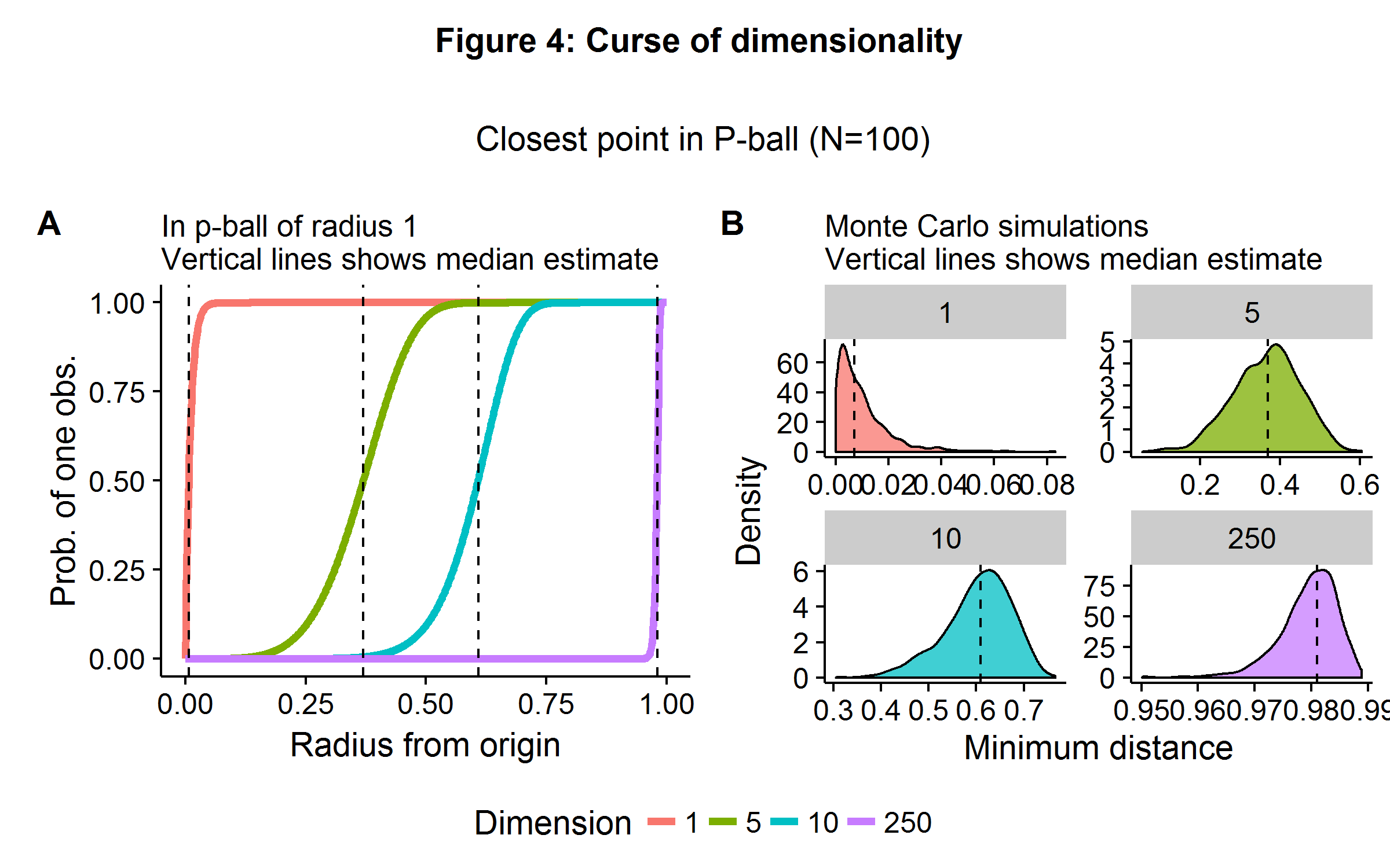
While machine learning techniques are able to ameliorate the \(p \gg N\) problem, they are not able to change the rules of geometry. The curse of dimensionality refers to a broad set of phenomena that occur in high-dimensional space. In statistics and machine learning, the problem presents itself when algorithms are only able to approximate some objective function by using “nearby” points. In high-dimensional space, it is almost always the case that no observations will be be very “close” to each other. Both theory and a Monte Carlo simulation quickly reveal the scope of the problem. Consider a unit \(p\)-ball, which has a radius of 1 (and where \(p=2\) is a circle and \(p=3\) is a sphere), and the origin is our point of perspective. If points are generated uniformly in this space (equal probability everywhere) then the probability of an observation less than or equal to a distance \(d\) away is \(1-(1-d^p)^n\).
Figure 4 below illustrates the theoretical and simulated results in the case of \(n=100\) observations and a dimensionality of \(p={ 1,5,10,250 }\). In 1-dimensional space, one only need move about 1% (on average) of the distance away from the origin to find another observation. In \(\mathbb{R}^5\), this jumps up to 40%. When there are \(250\) features, we would need to travel 98% of the range of each coordinate direction to find another observation (on average).
The curse of dimensionality highlights the problems that will arise when we are trying to match observations in high dimensional space. In such situations, comparing the difference in outcome between “similar” observations will prove a challenge and will need to be coupled with additional strategies. Such challenges occur for propensity score matching in large-\(p\) medical data sets, as it is difficult to match patients with similar features due to the geometric problems highlighted above. Several machine learning/statistical algorithms exist for paring down the number of features to a choice set using a data-driven approach. It should be noted that some of these algorithms appeal to sparsity (\(\textbf{s}\)): the number of causal feature weights is less than the number of observations (3).
\[\begin{align*} \textbf{s} = ||\boldsymbol\beta ||_0 = \sum_{i=1}^p I(\beta_p \neq 0) \ll n \hspace{1cm} (3) \end{align*}\]Or approximate sparsity: there is finite sample model error, but it is asymptotically zero (4).
\[\begin{align*} \frac{\textbf{s} \cdot \log p}{n} \to 0 \hspace{1cm} (4) \end{align*}\]Background #4: Regularization with the L1-norm
If sparsity is a plausible assumption, then a slight modification of the PRSS minimization problem seen in equation (2) by using the L1-norm instead of the L2-norm as a measure of model complexity yields the LASSO estimator. LASSO has the attractive property that its solution path is equivalent to soft thresholding: parameter values are either zero, or they are non-zero but have some shrinkage (like ridge regression).
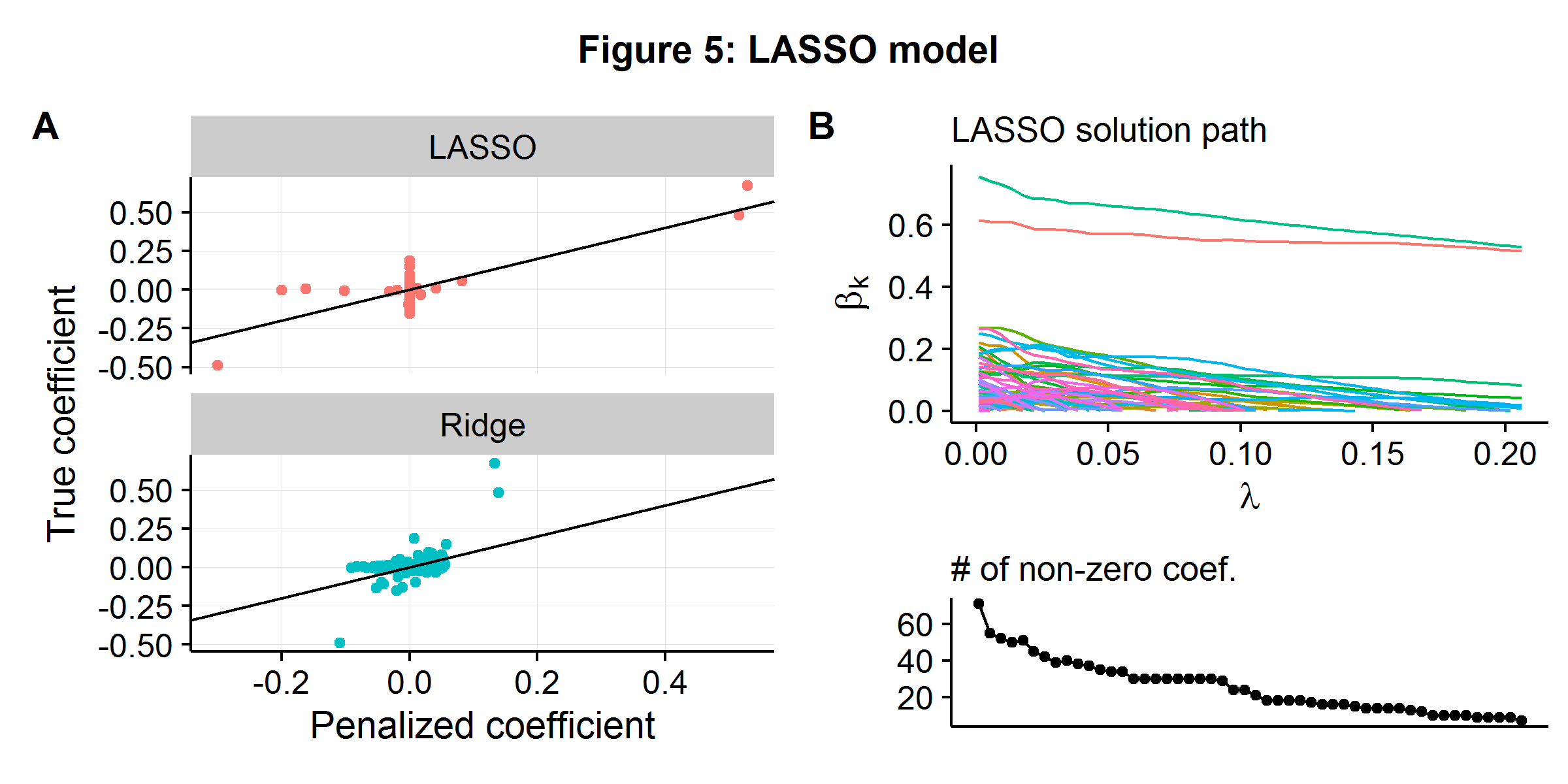
\[\begin{align*} \boldsymbol\beta_{\text{LASSO}} &= \arg\min_{\boldsymbol\beta} \hspace{2mm} \| \textbf{y} - \textbf{X}\boldsymbol\beta\|^2 + \lambda \|\boldsymbol\beta \|_1 \\ &= \arg\min_{\boldsymbol\beta} \hspace{2mm} RSS(\boldsymbol\beta) + \lambda \sum_{i=1}^p |\beta_i| \end{align*}\]Using the well-discussed data generating process from the above examples (\(n=100\) and \(p=250\)), we compare how ridge regression and LASSO work in practice. Data is generated using geometrically declining variance \(r=2\), and the hyperparameter \(\lambda\) is selected using (approximate) cross-validation for both models. Figure 5A below shows the relationship between the estimated and true coefficient weights for the two models. A large “blob” of coefficients are slightly above and below zero for ridge regression, with the three coefficients which have significant weights being systematically underestimated (as they are above/below the 45 degree line). In contrast, LASSO forces most of the coefficients to zero (even though they do have “some” causal weight), but more accurately estimates the causal parameters that have a larger effect. Figure 5B shows the LASSO algorithm’s solution path as the penalty against model complexity increases. As \(\lambda\) increases more and more parameters are “shut-off”. By the time \(\lambda\) reaches the value that minimizes the CV error (the last point), only 7 of the 250 potential features are in use.
If prediction accuracy is the only metric under consideration, then whether a sparse or highly shrunken model performs perform better will depend on the nature of the underlying data generating process. Models that contain embedded feature selection techniques, such as LASSO, will clearly prove more advantageous in environments where the goal is to pare down the number of features for either matching or causal inference. However, models like LASSO will still lead to biased coefficient estimates as the algorithm’s goal remains to minimize prediction error by trading off some measure of bias and variance, and hence still leading to bias.
Model #1: Double machine learning for causal inference
In a clinical setting one may be interested in estimating a parameter \(\theta\) for some treatment variable \(d_i\), while controlling for a vector of covariates which are often called “confounders”. For the rest of the discussion, it will be assumed that the outcome variable has a partially-linear model form:
\[\begin{align*} \underbrace{y_i}_{\text{outcome}} = \underbrace{d_i}_{\text{treatment}} \cdot \underbrace{\theta}_{\text{effect}} + \underbrace{g(\textbf{X}_i)}_{\text{confounders}} + \hspace{3mm} u_i \end{align*}\]When \(g: \hspace{2mm} \sum_{k=1}^p X_{ik}\beta_k\) this is a completely linear model. However \(g\) can be non-linear, and approximated by an algorithmic process: random forests, neural networks, LASSO, etc. If \(p \gg N\), the classical linear form of \(g\) will be insufficient for the reasons discussed above. A mistaken modelling strategy would be to force the two approaches together:
- Combine a machine learning algorithm for an over-determined feature set \(g(\textbf{X})\) with the simple linear addition of \(\textbf{d}\)
- Estimate \(\hat{\textbf{y}} = \textbf{d} \hat{\theta} + \hat{g}(\textbf{X})\)
- Report \(\hat{\theta}\) as the causal effect
When \(E ( \textbf{d} | \textbf{X} )=0\), this strategy is completely fine. However, in the presence of confounding, this strategy will no longer work as:
\[d_i = m(\textbf{X}_i) + v_i, \hspace{1cm} m: \mathbb{R}^p \to \mathbb{R}^1 \neq 0\]The estimate of \(\theta\) will now be biased as the machine learning algorithm embedded in \(g\) will apply some sort of regularization to the confounders, which will then lead to the treatment variable being correlated with the model residuals in some biased direction. Such a bias will occur in any dimensional setting including the classical \(N \gg p\) environment. For a motivating example, suppose \(n=1000\), \(p=20\), \(\theta=0.5\), only a few features impact both the outcome and the treatment, and the impact of the covariates is non-linear for both the outcome and the treatment. The true data generating process is shown below.
\[\begin{align*} y_i &= \theta d_i + \beta_1 \frac{1}{1+e^{-x_1}} + \beta_2 x_2 + u_i \\ d_i &= \gamma_1 \frac{1}{1+e^{-x_2}} + \gamma_2 x_1 + v_i \end{align*}\]Assuming the statistician is unaware of the true data generating process, flexible machine learning models can be deployed to approximate the unknown functional form such as random forests (an ensemble methods that combines decision trees with bagging). A naive, but intuitive, estimation strategy would be as follows:
- Initialize \(\hat{\theta}\) with a random number
- Apply a machine learning algorithm (random forests or LASSO) on residuals \(y_i - d_i\hat{\theta}= g(\textbf{X}_i)\) to get estimate of \(\hat{g}(\textbf{X}_i)\)
- Run a classical regression of \(y_i - \hat{g}(\textbf{X}_i) = d_i \theta\) to get estimate of \(\hat{\theta}\)
- Repeat Steps 2-3 until convergence
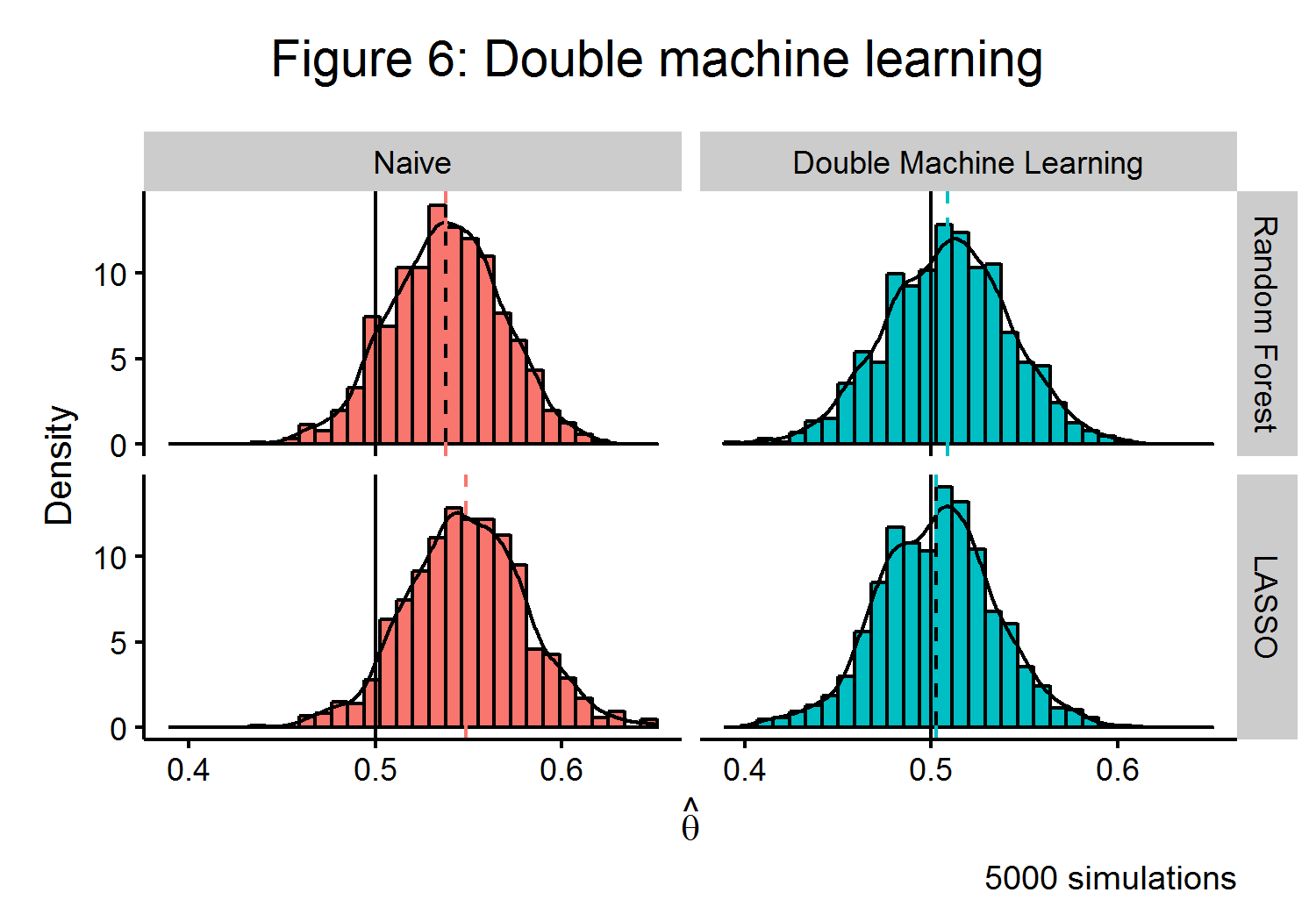
The left-hand side of Figure 6 shows that this naive estimator will have a clear bias when estimating \(\hat{\theta}\) in the presence of confounding. To overcome this problem, the ideal algorithmic approach would be to trade off between the bias and variance of an estimator and to control for any confounding. Double machine learning (DML) ((Chernozhukov and Newey 2016)) is one such recently developed strategy. The algorithm is able to use an orthogonalized formulation that partials out the effect of \(\textbf{X}\) from both \(\textbf{y}\) and \(\textbf{d}\). If \(\textbf{v} = \textbf{d} - m(\textbf{X})\) and \(\textbf{w} = \textbf{y} - m(\textbf{X})\theta + g(\textbf{X})\), then the approach of the DML estimator has a similar strategy to the classical Frisch-Waugh-Lovell estimator: \(\theta\) can be recovered by finding the part of \(\textbf{y}\) that cannot be explained by \(\textbf{X}\) from the part of \(\textbf{d}\) that cannot be explained by \(\textbf{X}\). The DML estimator also employs a clever use of sample splitting to help reduce bias.
\[\begin{align*} \hat{\theta}_{DML} &= \Big( \frac{1}{n} \sum_{i=1}^n \hat{v_i} \Big)^{-1} \frac{1}{n} \sum_{i=1}^n \hat{v_i}\hat{w_i} \end{align*}\]As the right-side of Figure 6 shows, this estimator is able to very closely approximate the true value of \(\theta\) for multiple machine learning algorithms. As the finite-sample bias of the DML estimator has a closed form, the extent of its bias is known to be bounded and can be shown to be root-\(n\) consistent under some mild conditions.
Model #2: Approximate residual balancing
An alternative formulation of estimating some causal parameter \(\theta\) in a partially linear model is to pose the question in terms of what the “average causal effect” of some treatment is. The Rubin Causal Framework (see (Rosembaum and Rubin 1983) and (Holland 1986)) considers the causal effect of a treatment to be the difference in outcome had the opposite treatment occurred, ceteris paribus. As a treatment can only be assigned once to a given person, the estimate of what would have occured must be imputed from the data. In a randomized control trial, the average difference between the (randomly) assigned treatment and non-treatment groups represents an unbiased estimate of the average treatment effect (ATE). In observational studies, treatment assigned will be correlated with other causal variables and hence the difference between the treatment/non-treatment groups (assuming a binary treatment option) will not represent a causal difference. However, if the unconfoundedness assumption holds[3], then tools exist to estimate the ATE in an observational study. For data sets which contain detailed medical and personal histories, the unconfoundedness assumption may only be plausible if the treatment variable is conditioned on a large number of features, which may exceed the number of observations.
When a propensity score (the probability of treatment assignment given baseline features) can be estimated, ATE can be inferred from either weighting outcomes by the inverse of the propensity score or matching patients from the different treatment groups that have a similar propensity score and averaging over their differences in outcome. While several approaches have been developed which use machine learning tools to estimate propensity scores or probability weights (see (McCaffrey and Morral 2004) and (Zubizarreta and Dylan 2015)), these methods are not guaranteed to achieve satisfactory performance as \(p\) increases as the curse of dimensionality makes it harder to “balance” observations as the feature space increases in rank.
The recently-developed approximate residual balancing (ARB) method (Athey Imbens and Wager 2016) provides a robust framework to estimate treatment effects in high dimensional space. It is implemented in a multi-stage process including fitting a regularized linear model, finding weights that approximately balance all the features, and then re-weighting the residuals. Simulations suggest that weights based on the balancing of residuals, as opposed to propensity scores, achieve better results when \(p \gg N\).
Formally the Rubin Causal Framework assumes that for each of the \(n\) observation there is a pair of potential outcomes \((Y_i(1),Y_i(0))\), a treatment indicator \(W_i \in {0,1}\), and a vector of features \(X_i \in \mathbb{R}^p\) where we allow for \(p \gg N\). A researcher therefore observes the following triple: \((X_i,W_i,Y_i^{obs})\), where:
\[Y_i^{obs} = Y_i(W_i) = \begin{cases} Y_i(1) & \text{if } W_i=1 \\ Y_i(0) & \text{if } W_i=0 \end{cases}\]The total number of treated and untreated units is \(n_t\) and \(n_c\), \(n = n_t + n_c\), with associated feature matrices denoted \(\textbf{X}_t\) and \(\textbf{X}_c\), respectively. The average treatment effect for the treated (ATT) is the average (theoretical) change in the outcome the patients who were treated received from getting the treatment, as equation 5 shows.
\[\begin{align*} \tau &= \frac{1}{n_t} \sum_{\{i: W_i=1\}} E[Y_i(1)-Y_i(0)|X_i] \hspace{1cm} (5) \end{align*}\]The ARB model assumes unconfoundedness and linearity in potential outcomes. While linearity is a strong assumption, a liberal inclusion of feature transformations is likely to be able to approximate even non-linear functions.
\[\begin{align*} W_i \hspace{2mm} &\text{independent} \hspace{2mm} (Y_i(1),Y_i(0)) \hspace{2mm} | \hspace{2mm} X_i \hspace{1cm} &\textbf{Unconfoundedness} \\ \mu_t(x_i) &= E[Y_i(1)|X_i=x_i] = x_i \beta_t \hspace{1cm} &\textbf{Linearity} \end{align*}\]Therefore the quantity of interest can be posed as finding some \(\beta_c\), such that it represents the true ATT:
\[\begin{align*} \tau &= \mu_t - \mu_c \\ &= \bar{\textbf{X}_t}\cdot \beta_t - \bar{\textbf{X}_t}\cdot \beta_c, \hspace{1cm} \bar{\textbf{X}_t} = \frac{1}{n_t} \sum_{\{i: W_i=1 \}}X_i \end{align*}\]The ARB algorithm has three steps:
- Compute the (positive) approximate weights \(\gamma\), where \(\zeta\) is a tuning parameter.
- Fit \(\hat{\beta_c}\) using an elastic net, which is a weighted average of LASSO and ridge penalty terms, and allows for both feature selection (like LASSO) but without necessarily throwing away correlated variables (like ridge regression). Note when \(\alpha=1\) (\(=0\)) the minimization problem is the same as the LASSO (ridge regression).
- Estimate the ATT.
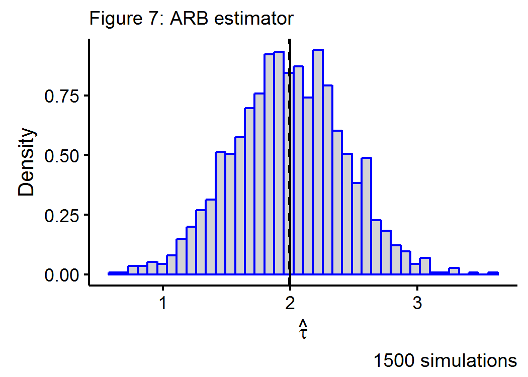
Figure 7 below shows the Monte Carlo simulations for a data generating process that has a true treatment effect of \(\tau=2\) in a \(n=100\), \(p=250\) environment, with a geometrically declining impact of the \(k^{th}\) covariate on the outcome.
References
Athey, and Imbens. 2016. "The State of Applied Econometrics-Causality and Policy Evaluation." In. https://arxiv.org/pdf/1607.00699v1.pdf.
Athey, Imbens, and Wager. 2016. "Approximate Residual Balancing: De-Biased Inference of Average Treatment Effects in High Dimensions." In. https://arxiv.org/pdf/1604.07125.pdf.
Belloni, Fernandez-Val, Chernozhukov, and Hansen. 2015. "Program Evaluation with High-Dimensional Data." In. https://stuff.mit.edu/~vchern/papers/slides_Late_August-2015_IFV.pd.
Breiman, Leo. 2001. "Statistical Modelling: Two Cultures." Statistical Science 16 (3): 199-233.
Chernozhukov, Demirer, Chetverikov, and Newey. 2016. "Double Machine Learning for Treatment and Causal Parameters." In. https://arxiv.org/abs/1608.00060.
Dai, Xue, Chen, and Yu. 2008. "Translated Learning: Transfer Learning Across Different Feature Spaces." In Advances in Neural Information Processing Systems 21, edited by D. Koller, D. Schuurmans, Y. Bengio, and L. Bottou, 353-60. http://books.nips.cc/papers/files/nips21/NIPS2008_0098.pdf.
Hoerl, Arthur. 1962. "Applications of Ridge Analysis to Regression Problems." Chemical Engineering Progress 58 (3): 54-59.
Holland, Paul. 1986. "Statistics and Causal Inference." Journal of the American Statistical Association 81 (396). [American Statistical Association, Taylor & Francis, Ltd.]: 945-60. http://www.jstor.org/stable/2289064.
McCaffrey, Ridgeway, and Morral. 2004. "Propensity Score Estimation with Boosted Regression for Evaluating Causal Effects in Observational Studies." Psychological Methods 9 (4): 403-25.
Rosembaum, and Rubin. 1983. "The Central Role of Propensity Score in Observational Studies for Causal Effects." Biometrika 70 (1): 41-55.
Zubizarreta, Imai, Gelman, and Dylan. 2015. "Stable Weights That Balance Covariates for Estimation with Incomplete Outcome Data." In.
-
A Bayesian believes that model parameters are themselves governed by a probability distribution. ↩
-
The difference between the algorithmic and statistical modelling approaches could be amusingly summarized as whether using your knuckles to determine which months have 31 days is sufficient to have “learned” something about the world. ↩
-
Conditional on each subject’s baseline features treatment assignment is as good as random. ↩