
miRNA data for species classification
Introduction
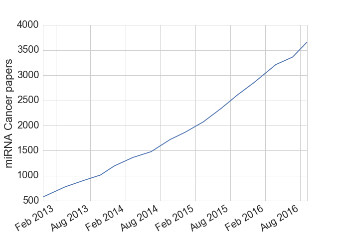
Micro RNAs (miRNAs) are a small RNA molecule, around 22 base pairs long[1], that are able to regulate gene expression by silencing specific RNAs. While these molecules were first discovered in the 1990s, their biological significance wasn’t fully appreciated until the early 2000s when they were found in C. elegans and Drosophola, the workhorse species of geneticists. Since then hundreds of miRNAs have been found in human genomes along with the discovery that a given miRNA can affect hundreds of other genes (i.e. they can bind with many types of RNA). Many cancer researchers are also interested in miRNAs due to their ability to inhibit tumor suppressor genes and act as effective oncogenes. Based on the data I downloaded from miRCancer, the cancer research community is averaging around two miRNA papers per day over the last several years.
Figure 1: miRNA text mining associations
In a recent Andrew Ng talk, Applying Deep Learning, he suggests that one way to become a better machine learning (ML) practitioner is to download existing studies, replicate the results, and see if you improve on anything. While a systems biology approach to modelling miRNA interactions will be the most successful in the long run, traditional ML techniques such as classification and dimensionality reduction will still have a role to play in this field. Because cell samples will usually contain more features (miRNA molecule types) than observations, predictive modelling will help to overcome the “large p, small n” problems stemming from these datasets.
Data: miRNA expression by species
After reading this ML project paper, I downloaded the miRNA expression data for various tissues in humans and mice here. The dataset contained 172 and 68 tissue samples for the two species, respectively, with 516 and 400 miRNA types for each. However, only 253 miRNAs were shared across the species so the dataset used in the modelling exercise was of this rank. The goal for the rest of this post is to use this dataset to develop a classification algorithm that will be able to successfully predict the species for a given sample. We begin by exploring the dataset, which has a numeric values for each miRNA type (miR-302a for example) in the columns, with a given row representing a sample from a specific tissue (liver for example).
num_both## # species miR-302a let-7g ... miR-20b miR-138 miR-376b
## 0 human 0.00000 0.00134 ... 0.01869 0.0 0.00000
## 1 human 0.00000 0.00000 ... 0.02920 0.0 0.000000
## .. ... ... ... ... ... ... ...
## 238 mouse 0.00000 0.02228 ... 0.00033 0.0 0.00000
## 239 mouse 0.00000 0.00000 ... 0.00000 0.0 0.00000The miRNA expression dataset can be visualized using a heatmap as Figure 2 shows below. As each column is a miRNA type, one can see that only a few molecules are expressed at a high level, and those that are tend to do so across multiple tissue types. However, most miRNA expression levels are close to “off”.
Figure 2: miRNA heatmap
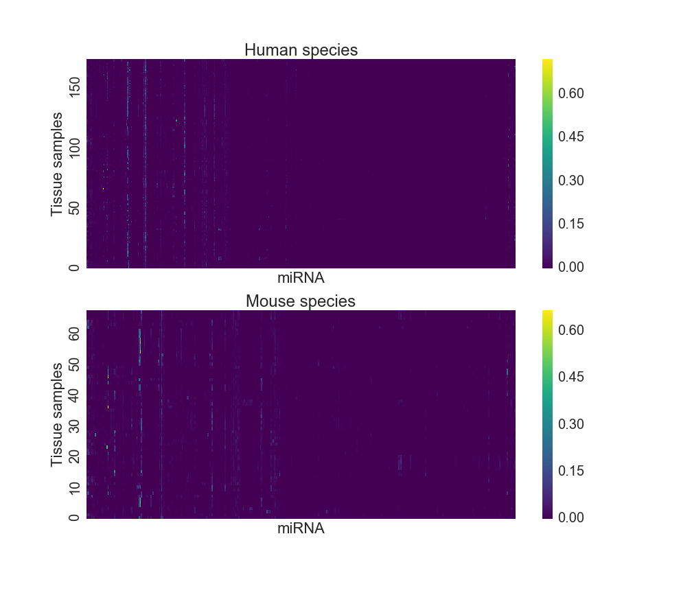
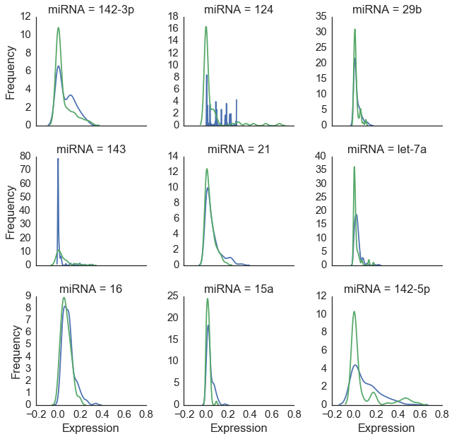
Figure 3 below shows a close-up view of nine miRNAs with the highest average expression levels. The distribution of values for these molecules is similar for humans and mice across tissues. While this points to our common ancestry with the little guys[2], it also presents a problem for classification as we will need some features to be differential expressed between our two species in order to successfully classify our observations[3].
Figure 3: Nine miRNA types with highest expression
Species classification: set up
In developing a classification rule, model parameters are determined on a “training set” and then evaluated on a “test set”. We randomly select 75% of the data to make up the training set, leaving 60 observations for validation. Partitioning data into these sets is crucial for developing a model which is robust to overfitting. Models that perform extremely well on training data may do poorly on test data due to their parameters “tuning to the noise” of the training data, while failing to “learn” the true patterns of the underlying data generating process.
In this dataset, human samples outnumber mice almost 3:1, and therefore bootstrapped samples from the mouse observations in the training data are generated to ensure an equal weighting of training performance between the two species, as there is no reason to believe the classifier should be biased toward either animal. The training dataset is of dimension 248x252, meaning there are more variables than observations, making this a classic “large p, small n” problem susceptible to overfitting without some intelligent intervention.
Discriminant function analysis
An extremely simple class of models used in classification are linear and quadratic discriminant analysis, denoted LDA and QDA. In these models, the likelihood of the data \(X\) is structured as a multivariate Gaussian distribution conditional for \(k\) different categories: \(f_k(X)\sim \frac{1}{(2n)^\pi |\Sigma|^{1/2}} \exp \Big(-\frac{1}{2} (X-\mu_k)^T\Sigma^{-1}_k (X-\mu_k) \Big)\).
In QDA, the covariance matrices are allowed to differ (\(\Sigma_k\)) between categories. In our context, we are saying that the probability of observing a given vector of features (of length 252 as noted above) can be evaluated under two distributions, whose moments are estimated from the data. A classification rule can be developed where the category whose distribution suggests a higher likelihood is chosen.
The sklearn module in Python is used throughout this post - the details of which can be found here. A naive LDA is used as a motivating example:
# Vanilla LDA
from sklearn.discriminant_analysis import LinearDiscriminantAnalysis
lda_fit = LinearDiscriminantAnalysis(solver='svd').fit(X_train,y_train)
train_acc = lda_fit.score(X_train,y_train)
test_acc = lda_fit.score(X_test,y_test)
print('Training accuracy is %0.1f%% and test accuracy is %0.1f%%' %
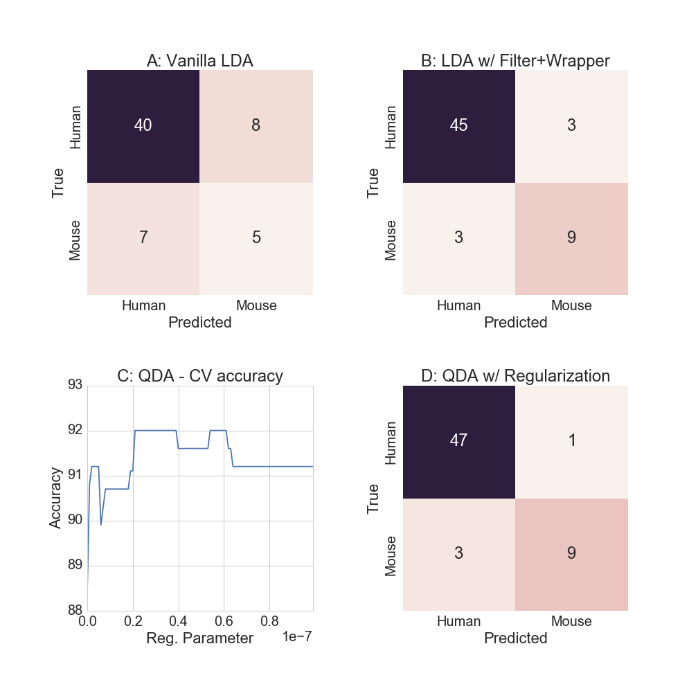
(round(train_acc*100), round(test_acc*100)) )## Training accuracy is 100.0% and test accuracy is 75.0%While the training accuracy is 100% (!) the test set accuracy falls to 75%[4]. Because there are more variables than observations, the model parameters are able to “perfectly” represent the training data. Also note that while the test accuracy for predicting humans was 85%, conditional mouse accuracy is a low 38.5%, as the confusion matrix shows in Figure 4A below.
The goals are now twofold: (i) improve the model accuracy beyond 75%, and (ii) improve the relative mouse predicting accuracy to better than a coin toss. To reduce the problem of overfitting, the discriminant function analysis models will take advantage of two concepts in machine learning.
- Filter methods: use characteristics of the data to select feature subsets
- Wrapper methods: use training set model performance to select features
In binary classification, the distribution of features needs to differ, in some way, between the two groups to have a good classifier. Filtering methods remove any variables that appear “uninteresting” by simple metrics such as t-tests. To combine a filtering and a wrapper method simultaneously, we will use a p-value cutoff of 1% to reduce our variable space and define an ordering of interesting variables[5], and then sequentially add features in order of the p-value score and test model accuracy using 10-fold cross-validation on the training data. It is important that we do not compare feature choice accuracy on the test set as this will allow the problem of overfitting to reemerge as the parameters would now be tuning to the noise contained in the test set. The purpose of the test set is that it is an independent sample of the data, and its information content must remain hidden until the final testing procedure.
# LDA with feature selection
tt = X_train.apply(lambda x: stats.ttest_ind(x[y_train==1],
    x[y_train!=1],equal_var=False).pvalue,axis=0).dropna()
p_cut = 0.01
tt_order = tt[tt<p_cut].sort_values().index
tt_score = np.repeat(np.NAN,tt_order.size)

# Run algorithm
for k in range(len(tt_order)):
    tt_cv = cross_validation.cross_val_score(lda,
            X_train[tt_order[range(k+1)]],y_train,cv=10).mean()
    tt_score[k] = tt_cv
n_tt = pd.Series(np.where(tt_score==tt_score.max())[0])
n_tt = n_tt[0]
print('Select the first %i features' % n_tt)
X_train2 = X_train[tt_order[0:n_tt]]
X_test2 = X_test[tt_order[0:n_tt]]
lda_fit2 = lda.fit(X_train2,y_train)
train_acc = lda_fit2.score(X_train2,y_train)
test_acc = lda_fit2.score(X_test2,y_test)
print('Training accuracy is %0.1f%% and test accuracy is %0.1f%%' %
      (round(train_acc*100), round(test_acc*100)) )
## Select the first 57 features
## Training accuracy is 94.0% and test accuracy is 90.0%Good improvement! While training sample accuracy declined to 94%, the test set accuracy (which is what is ultimately cared about) rose to 90%. As the confusion matrix shows in Figure 4B, we are now predicting 75% of the mouse labels accurately.
QDA and regularization
There are still techniques in the ML toolkit to improve test set performance: (i) use a new model, and (ii) use regularization (i.e. any technique which penalizes model complexity). Unlike LDA, QDA allows for non-linear relationships to be expressed. Additionally, as there was a 4% gap between the training/test set performance with LDA, this suggests that we can continue to move along the variance/ bias tradeoff curve.
The optimal regularization parameter is determined by using 10-fold cross validation on the training data. While multiple values of the regularization parameter achieve 92% CV accuracy, as Figure 4C shows, the largest one is chosen to reduce the chances of overfitting.
# QDA with regularization
X_train3 = X_train2.reset_index().drop('index',axis=1)
X_test3 = X_test2
shrink_par = np.arange(0,0.01,0.0001)/100000
shrink_acc = np.repeat(np.NaN,shrink_par.size*10).reshape([shrink_par.size,10])
from sklearn.cross_validation import KFold
kf = KFold(n=X_train2.shape[0],n_folds=10)
for row in range(len(shrink_par)):
    sp = shrink_par[row]
    qda_shrink = QuadraticDiscriminantAnalysis(reg_param=sp)
    col = 0
    for train_i, test_i in kf:
        acc = qda_shrink.fit(X_train3.loc[train_i],
                       y_train[train_i]).score(X_train3.loc[test_i],y_train[test_i])
        shrink_acc[row,col] = acc
        col += 1
av_cv = pd.DataFrame(shrink_acc).apply(lambda x: np.mean(x),axis=1)
reg_par_qda = shrink_par[max(np.where(av_cv==max(av_cv))[0])]

# Now fit the model
qda_reg = QuadraticDiscriminantAnalysis(reg_param=reg_par_qda)
qda_reg_fit = qda_reg.fit(X_train3,y_train)
train_acc3 = qda_reg_fit.score(X_train3,y_train)
test_acc3 = qda_reg_fit.score(X_test3,y_test)
y_qda_reg = qda_reg_fit.predict(X_test3)
print('Training accuracy is %0.1f%% and test accuracy is %0.1f%%' %
      (round(train_acc3*100), round(test_acc3*100)) )
Training accuracy is 96.0% and test accuracy is 93.0%As Figure 4D shows, almost all of the human examples are classified correctly, but the relative mouse accuracy remains unchanged.
Figure 4: Discriminant function analysis models
A better model yet?
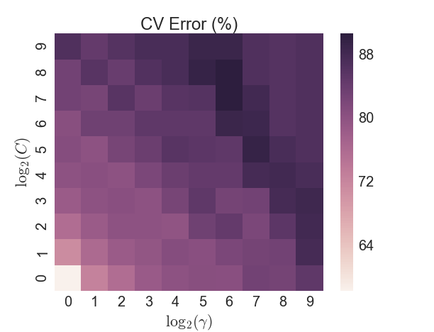
Another popular classifier is a Support Vector Machine (SVM), which transforms the data in such a way that a hyperplane can separate the two categories. An initial test of a SVM with a linear kernel yielded poor results, so the non-linear radial basis function (RBF) kernel was used (also known as the Gaussian kernel). The RBF is parameterized by a single variable \(\gamma\), in addition to selecting the penalty value \(C\) for the error term. A brute-force grid search approach was taken on a 5-fold CV split of the training data. However the in-sample accuracy was never able to exceed 90%, as Figure 5 shows, and the test sample accuracy lagged the LDA/QDA models.
Figure 5: SVM - CV error by parameter search
Summary
While other classifiers exist which could employed to see if the 93% accuracy could be exceeded, this post has covered enough ground to highlight two important concepts:
- The ML toolkit of filtering + wrapping + regularization + model selection is able to significantly improve prediciton accuracy
- miRNA datasets contain enough biological signals to be able to classify species with high accuracy
While correctly predicting the difference between humans and mice is in some sense trivial, the exercise highlights the value of miRNA datasets for other and more important questions in biology including determining the disease state of cells. As more and more miRNA sequencing data becomes available, ML models will become more powerful and able to provide stronger insights into biological problems.
-
The average human genome has more than 3 billion, to put this number in perspective. ↩
-
Our last common ancestor with mice was about 100 million years ago. ↩
-
However there may be non-linear combinations of the data within these nine genes that would be able to successfully differentiate the species. ↩
-
Using leave-one-out cross-validation achieves an accuracy of 72%, and a better conditional accuracy between the species of 76% and 61%, respectively. ↩
-
At this threshold, the number of variables is reduced to 63. ↩